Gamma-gamma Model#

In this notebook we show how to fit a Gamma-Gamma model in PyMC-Marketing. The model is presented in the paper: Fader, P. S., & Hardie, B. G. (2013). The Gamma-Gamma model of monetary value. February, 2, 1-9.

Prepare Notebook#

import arviz as az
import arviz_plots as azp
import matplotlib.pyplot as plt
import pandas as pd

from pymc_marketing import clv

# Plotting configuration
az.style.use("arviz-darkgrid")
plt.rcParams["figure.figsize"] = [10, 6]
plt.rcParams["figure.dpi"] = 100
plt.rcParams["figure.facecolor"] = "white"

%load_ext autoreload
%autoreload 2
%config InlineBackend.figure_format = "retina"

Load Data#

We start by loading the CDNOW dataset.

data_path = "https://raw.githubusercontent.com/pymc-labs/pymc-marketing/main/data/clv_quickstart.csv"

summary_with_money_value = pd.read_csv(data_path)
summary_with_money_value["customer_id"] = summary_with_money_value.index
summary_with_money_value.head()

	frequency	recency	T	monetary_value	customer_id
0	2	30.43	38.86	22.35	0
1	1	1.71	38.86	11.77	1
2	0	0.00	38.86	0.00	2
3	0	0.00	38.86	0.00	3
4	0	0.00	38.86	0.00	4

For the Gamma-Gamma model, we need to filter out customers who have made only one purchase.

returning_customers_summary = summary_with_money_value.query("frequency > 0")

returning_customers_summary.head()

	frequency	recency	T	monetary_value	customer_id
0	2	30.43	38.86	22.35	0
1	1	1.71	38.86	11.77	1
5	7	29.43	38.86	73.74	5
6	1	5.00	38.86	11.77	6
8	2	35.71	38.86	25.55	8

Model Specification#

Here we briefly describe the assumptions and the parametrization of the Gamma-Gamma model from the paper above.

The model of spend per transaction is based on the following three general assumptions:

The monetary value of a customer’s given transaction varies randomly around their average transaction value.
Average transaction values vary across customers but do not vary over time for any given individual.
The distribution of average transaction values across customers is independent of the transaction process.

For a customer with x transactions, let \(z_1, z_2, \ldots, z_x\) denote the value of each transaction. The customer’s observed average transaction value by

\[ \bar{z} = \frac{1}{x} \sum_{i=1}^{x} z_i \]

Now let’s describe the parametrization:

We assume that \(z_i \sim \text{Gamma}(p, ν)\), with \(E(Z_i| p, ν) = \xi = p/ν\).

– Given the convolution properties of the gamma, it follows that total spend across x transactions is distributed \(\text{Gamma}(px, ν)\).

– Given the scaling property of the gamma distribution, it follows that \(\bar{z} \sim \text{Gamma}(px, νx)\).
We assume \(ν \sim \text{Gamma}(q, \gamma)\).

We are interested in estimating the parameters \(p\), \(q\) and \(ν\).

Note

The Gamma-Gamma model assumes that there is no relationship between the monetary value and the purchase frequency. We can check this assumption by calculating the correlation between the average spend and the frequency of purchases.

returning_customers_summary[["monetary_value", "frequency"]].corr()

	monetary_value	frequency
monetary_value	1.000000	0.113884
frequency	0.113884	1.000000

The value of this correlation is close to \(0.11\), which in practice is considered low enough to proceed with the model.

PyMC-Marketing Implementation#

We can use the pre-built PyMC-Marketing implementation of the Gamma-Gamma model, which also provides nice plotting and prediction methods:

We can build the model so that we can see the model specification:

model = clv.GammaGammaModel()
model.build_model(data=returning_customers_summary)
model

Gamma-Gamma Model (Mean Transactions)
         p ~ Weibull(2, 1)
         q ~ Weibull(2, 1)
         v ~ Weibull(2, 10)
likelihood ~ Potential(f(q, p, v))

Note

It is not necessary to build the model before fitting it. We can fit the model directly.

Using MAP#

To begin with, lets use a numerical optimizer (L-BFGS-B) from scipy.optimize to find the maximum a posteriori (MAP) estimate of the parameters.

idata_map = model.fit(
    data=returning_customers_summary, method="map"
).posterior.ds.to_dataframe()

MAP ━━━━━━━━━━━━━━━━━━━━━━━━━━━━━━━━━━━━━━━━   0% 0:00:02 logp = -4,094.9, ||grad|| = 11.986

idata_map

		p	q	v
chain	draw
0	0	4.291772	3.64965	22.459997

MCMC#

We can also use MCMC to sample from the posterior distribution of the parameters. MCMC is a more robust method than MAP and provides uncertainty estimates for the parameters.

sampler_kwargs = {
    "draws": 2_000,
    "target_accept": 0.9,
    "chains": 4,
    "random_seed": 42,
}

idata_mcmc = model.fit(data=returning_customers_summary, **sampler_kwargs)

                                                                                                                   
                                                             Grad                                                  
  Progress               Draw        Divergen…   Step size   evals       Speed                Elapsed    Remaini…  
 ───────────────────────────────────────────────────────────────────────────────────────────────────────────────── 
  ━━━━━━━━━━━━━━━━━━━━   2400        0           0.356       11          1252.28 draws/s      0:00:01    0:00:00   
  ━━━━━━━━━━━━━━━━━━━━   2400        0           0.337       3           1284.07 draws/s      0:00:01    0:00:00   
  ━━━━━━━━━━━━━━━━━━━━   2400        0           0.318       3           1173.73 draws/s      0:00:02    0:00:00   
  ━━━━━━━━━━━━━━━━━━━━   2400        0           0.357       3           1202.45 draws/s      0:00:01    0:00:00

We can see some statistics of the posterior distribution of the parameters.

model.fit_summary()

	mean	sd	eti89_lb	eti89_ub	ess_bulk	ess_tail	r_hat	mcse_mean	mcse_sd
p	4.3	0.33	3.8	4.8	1758	2266	1.00	0.0079	0.0057
q	3.671	0.207	3.4	4	2237	2859	1.00	0.0044	0.003
v	22.7	2.56	19	27	1462	2031	1.00	0.067	0.048

Let’s visualize the posterior distributions and the rank plot:

We can compare the MCMC posterior with the MAP estimation.

pc = azp.plot_dist(
    idata_mcmc,
    var_names=["p", "q", "v"],
    point_estimate="mean",
    figure_kwargs={"figsize": (12, 4)},
)

for var_name in ["p", "q", "v"]:
    ax = pc.viz["plot"][var_name].item()
    ax.axvline(x=idata_map[var_name].item(), color="C2", linestyle="-.", label="MAP")
    ax.legend(loc="upper right")

pc.viz["figure"].item().suptitle(
    "Gamma-Gamma Model Parameters", fontsize=18, fontweight="bold", y=1.1
);

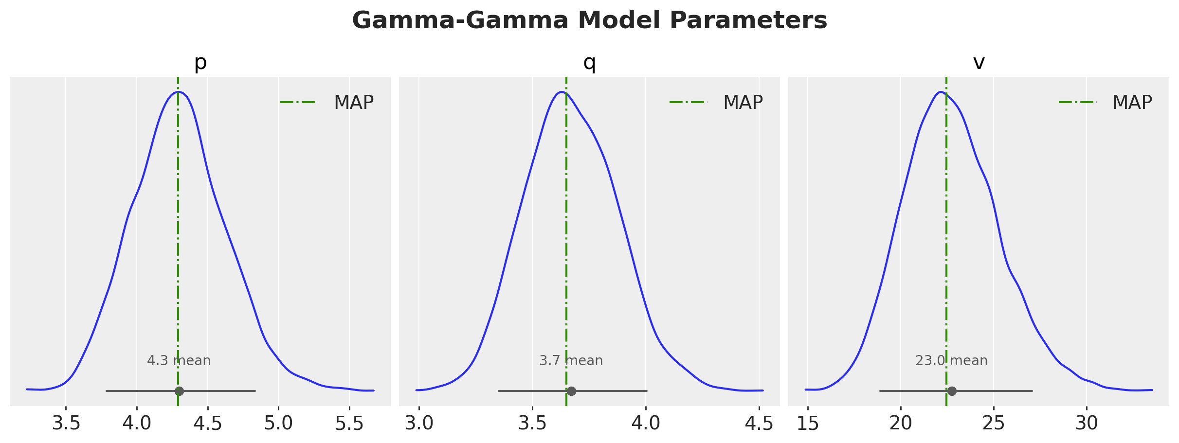
../../_images/47a2f2ef0902adcf629e7b0ca96967f75248e3fdcc1fadf441374740437f4176.png

We see that the MAP estimates are close to the mean of the posterior distribution obtained by MCMC.

Expected Customer Spend#

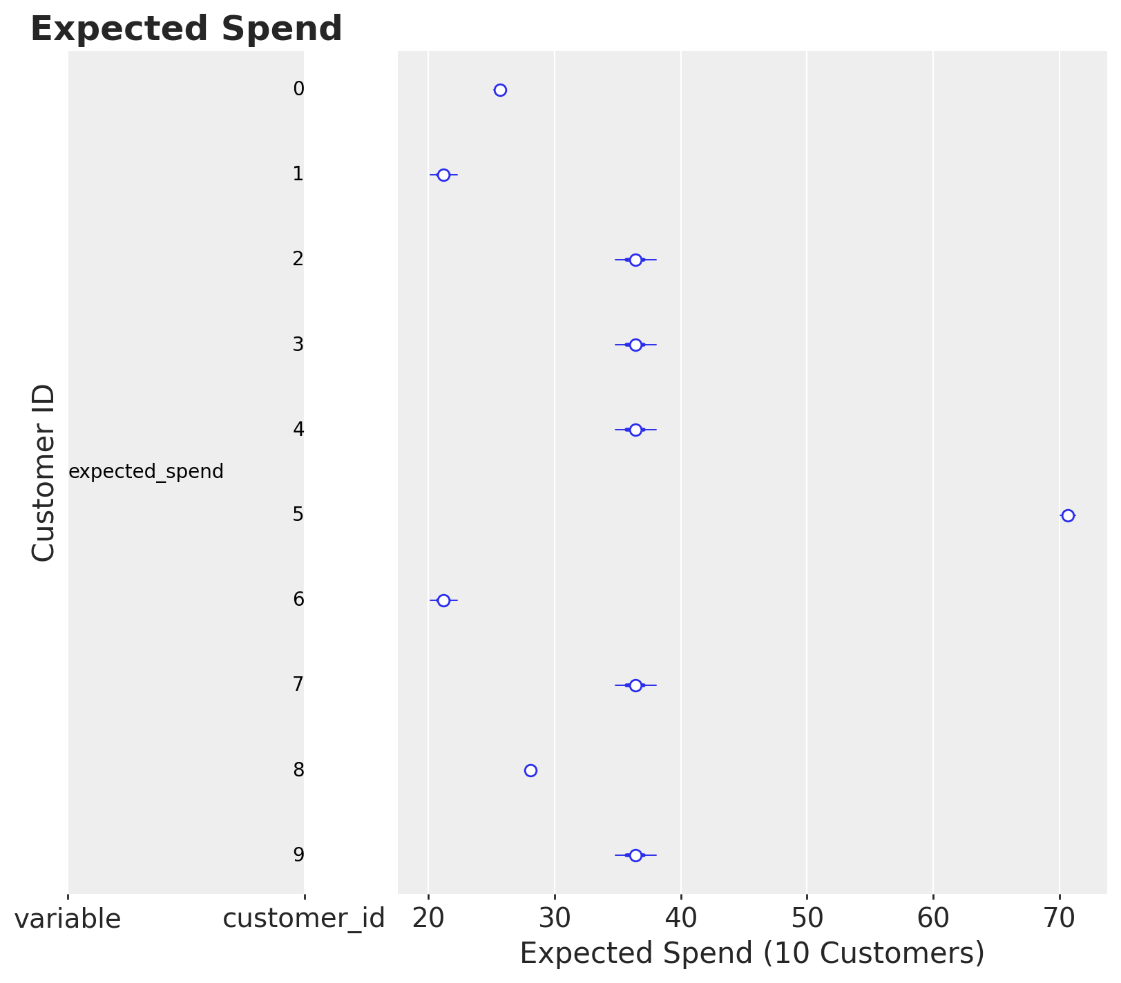
Once we have the posterior distribution of the parameters, we can use the expected_average_profit method to compute the conditional expectation of the average profit per transaction for a group of one or more customers.

expected_spend = model.expected_customer_spend(data=summary_with_money_value)

Let’s see how it looks for a subset of customers.

az.summary(expected_spend.isel(customer_id=range(10)), kind="stats")

	mean	sd	eti89_lb	eti89_ub
x[0]	26	0.31	25	26
x[1]	21	0.67	20	22
x[2]	36	1	35	38
x[3]	36	1	35	38
x[4]	36	1	35	38
x[5]	71	0.37	70	71
x[6]	21	0.67	20	22
x[7]	36	1	35	38
x[8]	28	0.27	28	29
x[9]	36	1	35	38

pc = azp.plot_forest(
    expected_spend.isel(customer_id=(range(10))).to_dataset(name="expected_spend"),
    combined=True,
    figure_kwargs={"figsize": (8, 7)},
)
label_ax, forest_ax = pc.viz["/"]["figure"].values.item().axes
forest_ax.set(xlabel="Expected Spend (10 Customers)")
label_ax.set(ylabel="Customer ID")
label_ax.set_title("Expected Spend", fontsize=18, fontweight="bold");

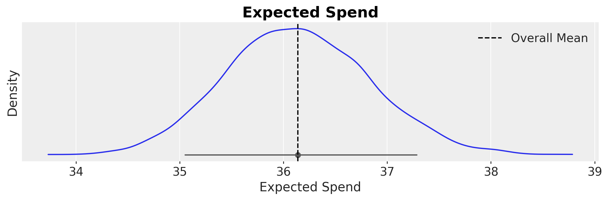
../../_images/7b8dee2ed2415012e1555b1e05df17e9c974a79cb159dcfa28db2fe91e08c56c.png

Finally, lets look at some statistics and the distribution for the whole dataset.

az.summary(expected_spend.mean("customer_id"), kind="stats")

	mean	sd	eti89_lb	eti89_ub
x	36	0.7	35	37

pc = azp.plot_dist(
    expected_spend.mean("customer_id").to_dataset(name="expected_spend"),
    visuals={"point_estimate_text": False},
)
ax = pc.viz["plot"]["expected_spend"].item()
ax.axvline(x=expected_spend.mean(), color="black", ls="--", label="Overall Mean")
ax.legend(loc="upper right")
ax.set(xlabel="Expected Spend", ylabel="Density")
ax.set_title("Expected Spend", fontsize=18, fontweight="bold");

../../_images/1b39d57a164a5f4ba41fa5a3b4687efcc83f386249eafc8bff69d9f4b43a322d.png

%load_ext watermark
%watermark -n -u -v -iv -w -p pymc_marketing,pymc,pytensor

Last updated: Mon, 13 Jul 2026

Python implementation: CPython
Python version       : 3.12.13
IPython version      : 9.15.0

pymc_marketing: 1.0.0.dev0
pymc          : 6.0.1
pytensor      : 3.0.7

arviz         : 1.2.0
arviz_plots   : 1.2.0
matplotlib    : 3.10.9
pandas        : 2.3.3
pymc_marketing: 1.0.0.dev0

Watermark: 2.6.0