Introduction to the Bass Diffusion Model

What is the Bass Model?

The Bass diffusion model, developed by Frank Bass in 1969, is a mathematical model that describes how new products get adopted in a population over time. It’s widely used in marketing to forecast sales of new products, especially when historical data is limited or non-existent.

The model captures the entire lifecycle of product adoption, from introduction to saturation, making it a powerful tool for product planning and marketing strategy development.

The Motivation Behind the Bass Model

Before the Bass model, companies struggled to predict the adoption patterns of new products. Traditional forecasting methods often failed because they couldn’t account for the social dynamics that drive product adoption. Frank Bass recognized that product adoption follows a distinct pattern:

• Initial slow growth: When a product first launches, adoption starts slowly

• Rapid acceleration: As more people adopt, word-of-mouth spreads and adoption accelerates

• Eventual saturation: Eventually, the market becomes saturated and adoption slows down

The Bass model provides a mathematical framework to capture these patterns, enabling businesses to make more informed decisions about production planning, inventory management, and marketing resource allocation.

Mathematical Formulation

The Bass model is based on a differential equation that describes the rate of adoption:

\[\frac{f(t)}{1-F(t)} = p + q F(t)\]

Where:

• \(F(t)\) is the installed base fraction (cumulative proportion of adopters)

• \(f(t)\) is the rate of change of the installed base fraction (\(f(t) = F'(t)\))

• \(p\) is the coefficient of innovation or external influence

• \(q\) is the coefficient of imitation or internal influence

The solution to this equation gives the adoption curve:

\[F(t) = \frac{1 - e^{-(p+q)t}}{1 + (\frac{q}{p})e^{-(p+q)t}}\]

The adoption rate at time \(t\) is given by:

\[f(t) = (p + q F(t))(1 - F(t))\]

Alternatively, this can be written as:

\[f(t) = \frac{(p+q)^2 \cdot e^{-(p+q)t}}{p \cdot (1+\frac{q}{p}e^{-(p+q)t})^2}\]

Key Components of the Bass Model Implementation

The Bass model implementation in PyMC-Marketing consists of several key components:

1. Adopters - The number of new adoptions at time \(t\):

\[\text{adopters}(t) = m \cdot f(p, q, t)\]

2. Innovators - Adoptions driven by external influence (advertising, etc.):

\[\text{innovators}(t) = m \cdot p \cdot (1 - F(p, q, t))\]

3. Imitators - Adoptions driven by internal influence (word-of-mouth):

\[\text{imitators}(t) = m \cdot q \cdot F(p, q, t) \cdot (1 - F(p, q, t))\]

4. Peak Adoption Time - When the adoption rate reaches its maximum:

\[\text{peak} = \frac{\ln(q) - \ln(p)}{p + q}\]

The total number of adopters over time is the sum of innovators and imitators, which equals \(\text{adopters}(t)\). All of these components are directly implemented in the PyMC model, allowing us to analyze each aspect of the diffusion process separately.

Understanding the Relationship Between Components

A key insight of the Bass model is how it decomposes adoption into two sources:

\[\text{adopters}(t) = \text{innovators}(t) + \text{imitators}(t)\]

At each time point:

• Innovators (\(m \cdot p \cdot (1 - F(t))\)) represents new adoptions coming from people who are influenced by external factors like advertising

• Imitators (\(m \cdot q \cdot F(t) \cdot (1 - F(t))\)) represents new adoptions coming from people who are influenced by previous adopters

As time progresses:

• Initially, innovators dominate the adoption process when few people have adopted (\(F(t)\) is small)

• Later, imitators become the primary source of new adoptions as the word-of-mouth effect grows

• Eventually, both decrease as the market approaches saturation (\(F(t)\) approaches 1)

The cumulative adoption at any time point is:

\[\text{Cumulative Adoption}(t) = m \cdot F(t)\]

This means that as \(t \to \infty\), the cumulative adoption approaches the total market potential \(m\):

\[\lim_{t \to \infty} \text{Cumulative Adoption}(t) = m\]

Therefore, the Bass model provides a complete accounting of the market:

• At each time point, new adopters are either innovators or imitators

• Over the entire product lifecycle, all potential adopters (m) eventually adopt the product

• The model tracks both the adoption rate (new adopters per time period) and the cumulative adoption (total adopters to date)

This structure enables marketers to understand not just how many people will adopt over time, but also the driving forces behind adoption at different stages of the product lifecycle.

Understanding the Key Parameters

The model has three main parameters:

• Market potential (m): Total number of eventual adopters (the ultimate market size)

• Innovation coefficient (p): Measures external influence like advertising and media - typically \(0.01-0.03\)

• Imitation coefficient (q): Measures internal influence like word-of-mouth - typically \(0.3-0.5\)

Parameter Interpretation

• A higher p value indicates stronger external influence (advertising, marketing)

• A higher q value indicates stronger internal influence (word-of-mouth, social interactions)

• The ratio q/p indicates the relative strength of internal vs. external influences

• The peak of adoption occurs at time

\[t^* = \frac{\ln(q / p)}{p + q}\]

Innovators vs. Imitators

The Bass model distinguishes between two types of adopters:

1. Innovators: People who adopt independently of others’ decisions, influenced mainly by mass media and external communications

   • Mathematically represented as: \(\text{innovators}(t) = m \cdot p \cdot (1 - F(p, q, t))\)

2. Imitators: People who adopt because of social influence and word-of-mouth from previous adopters

   • Mathematically represented as: \(\text{imitators}(t) = m \cdot q \cdot F(p, q, t) \cdot (1 - F(p, q, t))\)

Real-World Applications

The Bass model has been successfully applied to forecast the adoption of various products and technologies:

• Consumer durables: TVs, refrigerators, washing machines

• Technology products: Smartphones, computers, software

• Pharmaceutical products: New drugs and treatments

• Entertainment products: Movies, games, streaming services

• Services and subscriptions: Banking services, subscription plans

Business Value: Why the Bass Model Matters to Executives and Marketers

From a business perspective, the Bass diffusion model provides substantial competitive advantages and ROI benefits:

1. Resource Optimization and Cash Flow Management

• Production Planning: Avoid costly overproduction or stockouts by accurately forecasting demand curves

• Marketing Budget Allocation: Optimize spending across the product lifecycle, investing more during key inflection points

• Supply Chain Efficiency: Coordinate with suppliers and distributors based on predicted adoption rates

• Cash Flow Optimization: Better predict revenue streams, improving financial planning and investor relations

2. Strategic Decision Making

• Launch Timing: Determine the optimal time to enter a market based on diffusion patterns

• Pricing Strategy: Implement dynamic pricing strategies aligned with the adoption curve

• Competitive Analysis: Compare your product’s adoption parameters with competitors to identify strengths and weaknesses

• Product Portfolio Management: Make informed decisions about when to phase out older products and introduce new ones

3. Risk Mitigation

• Scenario Planning: Test different market assumptions and external factors through parameter variations

• Early Warning System: Identify deviations from expected adoption curves early, enabling faster intervention

• Investment Justification: Provide data-driven forecasts to justify R&D and marketing investments to stakeholders

4. Performance Measurement

• Marketing Effectiveness: Measure the impact of marketing campaigns on the innovation coefficient (p)

• Word-of-Mouth Strength: Quantify the power of your brand’s social influence through the imitation coefficient (q)

• Total Market Potential: Validate or adjust your total addressable market estimates (m)

In today’s data-driven business environment, companies that effectively utilize models like Bass diffusion gain a significant competitive edge through more precise forecasting, better resource allocation, and strategic market timing.

Bayesian Extensions

In this notebook, we show how to generate simulated data from the Bass model and fit a Bayesian model to it. The Bayesian formulation offers several advantages:

• Uncertainty quantification through prior distributions on parameters

• Hierarchical modeling for multiple products or markets

• Incorporation of expert knowledge through informative priors

• Full probability distributions for future adoption forecasts

What we’ll do in this notebook

In this notebook, we’ll:

1. Set up parameters for a Bass model simulation

2. Generate simulated adoption data for multiple products

3. Fit the Bass model to our simulated data with the BassModel class

4. Visualize the adoption curves with the built-in plotting methods

5. Forecast adoption beyond the observed window

6. Save and load the fitted model

7. Track the workflow with MLflow

Prepare Notebook

import tempfile
from typing import Any

import arviz as az
import arviz_plots as azp
import matplotlib.pyplot as plt
import numpy as np
import numpy.typing as npt
import pandas as pd
import pymc as pm
import xarray as xr
from pymc_extras.prior import Prior, Scaled

from pymc_marketing.bass import BassModel, create_bass_model
from pymc_marketing.plot import plot_curve

az.style.use("arviz-darkgrid")
plt.rcParams["figure.figsize"] = [12, 7]
plt.rcParams["figure.dpi"] = 100

%config InlineBackend.figure_format = "retina"

seed: int = sum(map(ord, "bass"))
rng: np.random.Generator = np.random.default_rng(seed=seed)

Setting Up Simulation Parameters

First, we’ll set up the parameters for our simulation. This includes:

• The time period for our simulation (in weeks)

• The number of products to simulate

• Start dates for the simulation period

def setup_simulation_parameters(
    n_weeks: int = 52,
    n_products: int = 9,
    start_date: str = "2023-01-01",
    cutoff_start_date: str = "2023-12-01",
) -> tuple[
    npt.NDArray[np.int_],
    pd.DatetimeIndex,
    pd.DatetimeIndex,
    list[str],
    pd.Series,
    dict[str, Any],
]:
    """Set up initial parameters for the Bass diffusion model simulation.

    Parameters
    ----------
    n_weeks : int
        Number of weeks to simulate
    n_products : int
        Number of products to include in the simulation
    start_date : str
        Starting date for the simulation period
    cutoff_start_date : str
        Latest possible start date for products

    Returns
    -------
    T : numpy.ndarray
        Time array (weeks)
    possible_dates : pandas.DatetimeIndex
        All dates in the simulation period
    possible_start_dates : pandas.DatetimeIndex
        Possible start dates for products
    products : list
        List of product names
    product_start : pandas.Series
        Start date for each product
    coords : dict
        Coordinates for PyMC model
    """
    # Set a seed for reproducibility
    seed = sum(map(ord, "bass"))
    rng = np.random.default_rng(seed)

    # Create time array and date range
    T = np.arange(n_weeks)
    possible_dates = pd.date_range(start_date, freq="W-MON", periods=n_weeks)
    cutoff_start_date = pd.to_datetime(cutoff_start_date)
    cutoff_start_date = cutoff_start_date + pd.DateOffset(weeks=1)
    possible_start_dates = possible_dates[possible_dates < cutoff_start_date]

    # Generate product names and random start dates
    products = [f"P{i}" for i in range(n_products)]
    product_start = pd.Series(
        rng.choice(possible_start_dates, size=len(products)),
        index=pd.Index(products, name="product"),
    )

    coords = {"T": T, "product": products}
    return T, possible_dates, possible_start_dates, products, product_start, coords

Creating Prior Distributions

For our Bayesian Bass model, we need to specify prior distributions for the key parameters:

• m (market potential): How many units can potentially be sold in total

• p (innovation coefficient): Rate of adoption from external influences

• q (imitation coefficient): Rate of adoption from internal/social influences

• likelihood: The probability distribution that models the observed adoption data

For the market potential m we use a scaling trick to specify a scale-free prior and then add a global factor:

def create_bass_priors(factor: float) -> dict[str, Prior | Scaled]:
    """Define prior distributions for the Bass model parameters.

    Returns
    -------
    dict
        Dictionary of prior distributions for m, p, q, and likelihood

    Notes
    -----
    - m: Market potential (scaled Gamma distribution)
    - p: Innovation coefficient (Beta distribution)
    - q: Imitation coefficient (Beta distribution)
    - likelihood: Observation model (Negative Binomial)
    """
    return {
        # We use a scaled Gamma distribution for the market potential.
        "m": Scaled(Prior("Gamma", mu=1, sigma=0.1, dims="product"), factor=factor),
        "p": Prior("Beta", mu=0.02, dims="product").constrain(lower=0.01, upper=0.03),
        "q": Prior("Beta", dims="product").constrain(lower=0.3, upper=0.5),
        "likelihood": Prior("NegativeBinomial", n=1.5, dims="product"),
    }

Let’s generate and visualize the priors.

FACTOR = 50_000
priors = create_bass_priors(factor=FACTOR)

fig, ax = plt.subplots(nrows=2, ncols=1, figsize=(15, 12))

priors["p"].preliz.plot_pdf(ax=ax[0])
ax[0].set(title="Innovation Coefficient (p)")
priors["q"].preliz.plot_pdf(ax=ax[1])
ax[1].set(title="Imitation Coefficient (q)")
fig.suptitle(
    "Prior Distributions for Bass Model Parameters",
    fontsize=18,
    fontweight="bold",
    y=0.95,
);

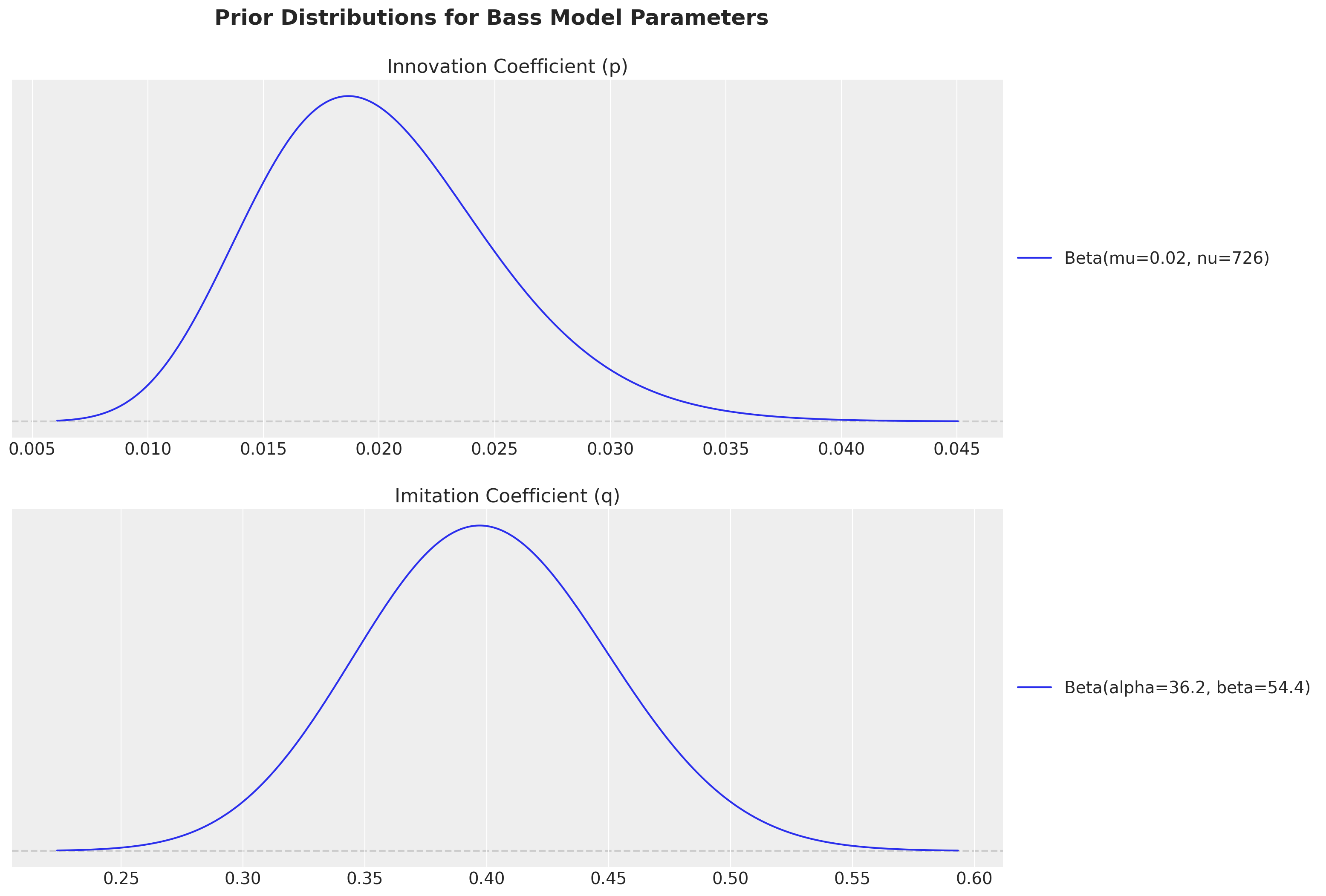
Observe we have chosen the priors within the usual ranges of empirical studies:

• Innovation coefficient (p): Measures external influence like advertising and media - typically \(0.01-0.03\)

• Imitation coefficient (q): Measures internal influence like word-of-mouth - typically \(0.3-0.5\)

Generate Synthetic Data

With the generative Bass model, we can generate a synthetic dataset by sampling from the prior and choosing one particular sample to use as observed data. For this purpose we define two auxiliary functions.

Here we use the lower-level create_bass_model() function, which returns a raw pm.Model. It is the right tool when you need direct access to the model object, for example to sample from the prior. For fitting we will use the higher-level BassModel class below.

def sample_prior_bass_data(model: pm.Model) -> xr.Dataset:
    """Generate a sample from the prior predictive distribution of the Bass model.

    Parameters
    ----------
    model : pymc.Model
        The PyMC model to sample from

    Returns
    -------
    xarray.Dataset
        One prior draw: the simulated ``y`` plus the true ``m``, ``p``, ``q``
    """
    with model:
        idata = pm.sample_prior_predictive(random_seed=rng)
    return idata["prior"].sel(chain=0, draw=0)


def transform_to_actual_dates(bass_data, product_start, possible_dates) -> pd.DataFrame:
    """Transform simulation data from time index to calendar dates.

    Parameters
    ----------
    bass_data : xarray.DataArray
        Simulated bass model data
    product_start : pandas.Series
        Start date for each product
    possible_dates : pandas.DatetimeIndex
        All dates in the simulation period

    Returns
    -------
    pandas.DataFrame
        Adoption data with actual calendar dates
    """
    bass_data = bass_data.to_dataset()
    bass_data["product_start"] = product_start.to_xarray()

    df_bass_data = (
        bass_data.to_dataframe().drop(columns=["chain", "draw"]).reset_index()
    )
    df_bass_data["actual_date"] = df_bass_data["product_start"] + pd.to_timedelta(
        7 * df_bass_data["T"], unit="days"
    )

    return (
        df_bass_data.set_index(["actual_date", "product"])
        .y.unstack(fill_value=0)
        .reindex(possible_dates, fill_value=0)
    )

Now we can generate the observed data:

# Setup simulation parameters
T, possible_dates, _, products, product_start, coords = setup_simulation_parameters()

# Create and configure the Bass model
generative_model = create_bass_model(t=T, coords=coords, observed=None, priors=priors)

# Sample and select one "observed" dataset.
prior_draw = sample_prior_bass_data(generative_model)
bass_data = prior_draw["y"]
actual_data = transform_to_actual_dates(bass_data, product_start, possible_dates)

Sampling: [m_unscaled, p, q, y]

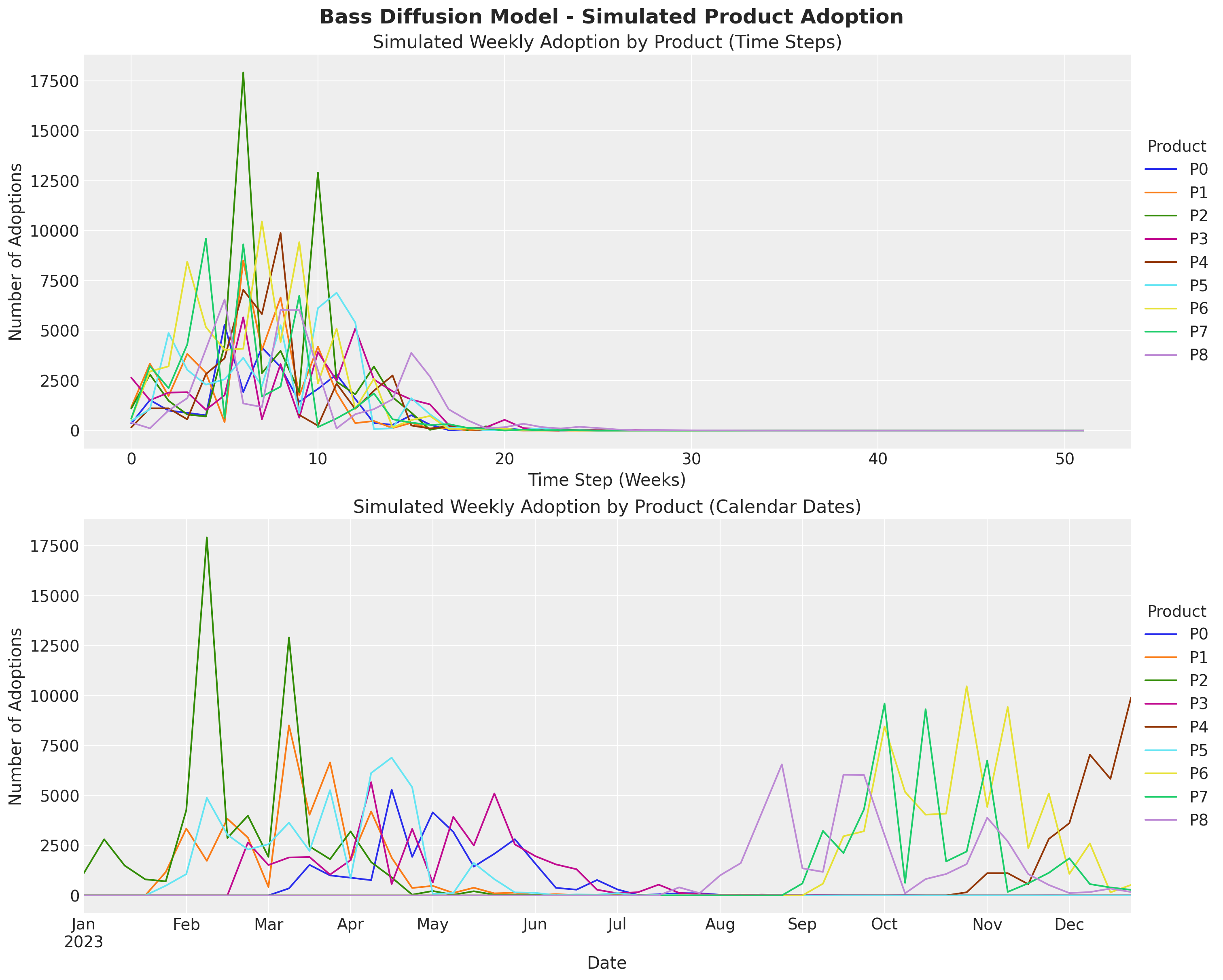
The actual_data data frame has the typical format of a real dataset.

actual_data

product	P0	P1	P2	P3	P4	P5	P6	P7	P8
2023-01-02	0	0	1100	0	0	0	0	0	0
2023-01-09	0	0	2808	0	0	0	0	0	0
2023-01-16	0	0	1491	0	0	0	0	0	0
2023-01-23	0	0	804	0	0	0	0	0	0
2023-01-30	0	1171	706	0	0	487	0	0	0
2023-02-06	0	3346	4268	0	0	1068	0	0	0
2023-02-13	0	1732	17916	0	0	4882	0	0	0
2023-02-20	0	3836	2874	0	0	3038	0	0	0
2023-02-27	0	2893	3989	2651	0	2298	0	0	0
2023-03-06	0	421	1929	1521	0	2562	0	0	0
2023-03-13	353	8508	12905	1899	0	3642	0	0	0
2023-03-20	1529	4036	2452	1922	0	2229	0	0	0
2023-03-27	1002	6654	1814	1040	0	5269	0	0	0
2023-04-03	887	1756	3204	1768	0	863	0	0	0
2023-04-10	765	4199	1668	5665	0	6125	0	0	0
2023-04-17	5294	1891	900	568	0	6895	0	0	0
2023-04-24	1929	374	37	3329	0	5409	0	0	0
2023-05-01	4157	478	223	645	0	74	0	0	0
2023-05-08	3180	125	31	3930	0	118	0	0	0
2023-05-15	1441	385	209	2500	0	1622	0	0	0
2023-05-22	2085	104	31	5103	0	814	0	0	0
2023-05-29	2812	134	38	2554	0	151	0	0	0
2023-06-05	1585	12	13	1964	0	128	0	0	0
2023-06-12	379	64	23	1552	0	13	0	0	0
2023-06-19	288	18	27	1312	0	49	0	0	0
2023-06-26	771	5	3	286	0	37	0	0	0
2023-07-03	297	15	3	105	0	117	0	0	0
2023-07-10	24	1	0	162	0	1	0	0	0
2023-07-17	55	0	0	539	0	24	0	0	0
2023-07-24	113	1	0	126	0	6	0	0	403
2023-07-31	109	0	0	64	0	6	0	0	114
2023-08-07	32	1	3	29	0	2	0	0	1008
2023-08-14	38	1	0	9	0	0	0	0	1619
2023-08-21	11	0	0	41	0	1	0	0	4079
2023-08-28	18	0	0	27	0	3	0	0	6557
2023-09-04	8	0	0	29	0	4	0	599	1357
2023-09-11	6	0	0	10	0	0	586	3228	1178
2023-09-18	3	0	0	4	0	1	2960	2122	6038
2023-09-25	0	0	0	5	0	1	3214	4308	6029
2023-10-02	1	0	0	1	0	0	8454	9599	3021
2023-10-09	5	0	0	6	0	0	5179	629	107
2023-10-16	0	0	0	0	0	0	4040	9317	819
2023-10-23	0	0	0	0	0	0	4095	1701	1072
2023-10-30	0	0	0	0	158	0	10464	2199	1567
2023-11-06	0	0	0	0	1113	0	4429	6746	3888
2023-11-13	0	0	0	0	1112	0	9427	176	2704
2023-11-20	0	0	0	0	562	0	2360	608	1065
2023-11-27	0	0	0	3	2826	0	5102	1129	524
2023-12-04	0	0	0	0	3614	0	1077	1859	119
2023-12-11	0	0	0	0	7042	0	2602	567	168
2023-12-18	0	0	0	0	5833	0	153	398	342
2023-12-25	0	0	0	0	9884	0	525	281	173

On the other hand, the bass_data has the same data as arrays indexed by time (relative) and product.

Let’s visualize both.

fig, ax = plt.subplots(
    nrows=2, ncols=1, figsize=(15, 12), sharex=False, sharey=True, layout="constrained"
)

# Plot raw simulated data (by time step)
bass_data.to_series().unstack().plot(ax=ax[0])
ax[0].legend(
    title="Product", title_fontsize=14, loc="center left", bbox_to_anchor=(1, 0.5)
)
ax[0].set(
    title="Simulated Weekly Adoption by Product (Time Steps)",
    xlabel="Time Step (Weeks)",
    ylabel="Number of Adoptions",
)

# Plot data with actual calendar dates
actual_data.plot(ax=ax[1])
ax[1].legend(
    title="Product", title_fontsize=14, loc="center left", bbox_to_anchor=(1, 0.5)
)
ax[1].set(
    title="Simulated Weekly Adoption by Product (Calendar Dates)",
    xlabel="Date",
    ylabel="Number of Adoptions",
)

fig.suptitle(
    "Bass Diffusion Model - Simulated Product Adoption", fontsize=18, fontweight="bold"
);

Fit the Model

We are now ready to fit the model. We use the BassModel class, a ModelBuilder subclass that wraps create_bass_model behind the standard .fit(), .save() and .load() workflow.

The priors go into model_config and the sampler settings into sampler_config. The fit method accepts the data as xr.Dataset (with an observed variable), a wide pd.DataFrame (one column per product), a pd.Series, or a np.ndarray; see to_bass_dataset() for the conversion rules. Here we pass the simulated data as a xr.Dataset.

observed_ds = bass_data.drop_vars(["chain", "draw"]).to_dataset(name="observed")

model = BassModel(
    model_config=priors,
    sampler_config={
        "tune": 1_500,
        "draws": 2_000,
        "chains": 4,
        "nuts_sampler": "nutpie",
        "compile_kwargs": {"mode": "NUMBA"},
    },
)

idata = model.fit(data=observed_ds, random_seed=rng)

model.sample_posterior_predictive(X=observed_ds, extend_idata=True, random_seed=rng);

NUTS[nutpie]: [m_unscaled, p, q]

Sampling: [y]

We do not have any divergences. Let’s look at the summary of the parameters.

az.summary(data=idata, var_names=["p", "q", "m"])

	mean	sd	eti89_lb	eti89_ub	ess_bulk	ess_tail	r_hat	mcse_mean	mcse_sd
p[P0]	0.0205	0.00441	0.014	0.028	6490	5644	1.00	5.5e-05	4.2e-05
p[P1]	0.024	0.00462	0.017	0.032	8216	5942	1.00	5.1e-05	3.8e-05
p[P2]	0.01866	0.0037	0.013	0.025	7329	6184	1.00	4.3e-05	3.2e-05
p[P3]	0.02032	0.00383	0.015	0.027	7339	5946	1.00	4.5e-05	3.5e-05
p[P4]	0.0194	0.00423	0.013	0.027	7077	5721	1.00	5e-05	3.9e-05
p[P5]	0.01991	0.00396	0.014	0.027	7037	5980	1.00	4.7e-05	3.7e-05
p[P6]	0.02327	0.00423	0.017	0.03	7516	6429	1.00	4.9e-05	3.7e-05
p[P7]	0.0243	0.00468	0.017	0.032	7184	5747	1.00	5.5e-05	4.2e-05
p[P8]	0.01585	0.00341	0.011	0.022	5851	5613	1.00	4.4e-05	3.4e-05
q[P0]	0.4165	0.0196	0.39	0.45	6527	5610	1.00	0.00024	0.00018
q[P1]	0.4855	0.022	0.45	0.52	8082	6659	1.00	0.00024	0.00017
q[P2]	0.4347	0.0191	0.4	0.47	7214	5906	1.00	0.00022	0.00015
q[P3]	0.35	0.0161	0.32	0.38	7220	5692	1.00	0.00019	0.00014
q[P4]	0.4254	0.0194	0.39	0.46	7190	6358	1.00	0.00023	0.00016
q[P5]	0.4014	0.0182	0.37	0.43	6612	5687	1.00	0.00022	0.00016
q[P6]	0.416	0.0185	0.39	0.45	7421	6187	1.00	0.00021	0.00015
q[P7]	0.4175	0.0195	0.39	0.45	6849	6046	1.00	0.00024	0.00017
q[P8]	0.3319	0.0159	0.31	0.36	5585	5140	1.00	0.00021	0.00015
m[P0]	5e+04	4e+03	39000	53000	13624	5886	1.00	38	26
m[P1]	5e+04	4e+03	42000	56000	13804	6128	1.00	39	27
m[P2]	5e+04	5e+03	45000	59000	14030	6223	1.00	39	28
m[P3]	5e+04	4e+03	43000	57000	12649	6003	1.00	40	28
m[P4]	5e+04	4e+03	40000	55000	13469	5790	1.00	39	27
m[P5]	5e+04	4e+03	43000	57000	12490	6331	1.00	40	28
m[P6]	5e+04	5e+03	45000	60000	15049	6402	1.00	37	26
m[P7]	5e+04	4e+03	43000	57000	11777	5689	1.00	41	30
m[P8]	5e+04	4e+03	43000	57000	13617	6345	1.00	38	27

azp.plot_trace_dist(idata, var_names=["p", "q", "m"]);

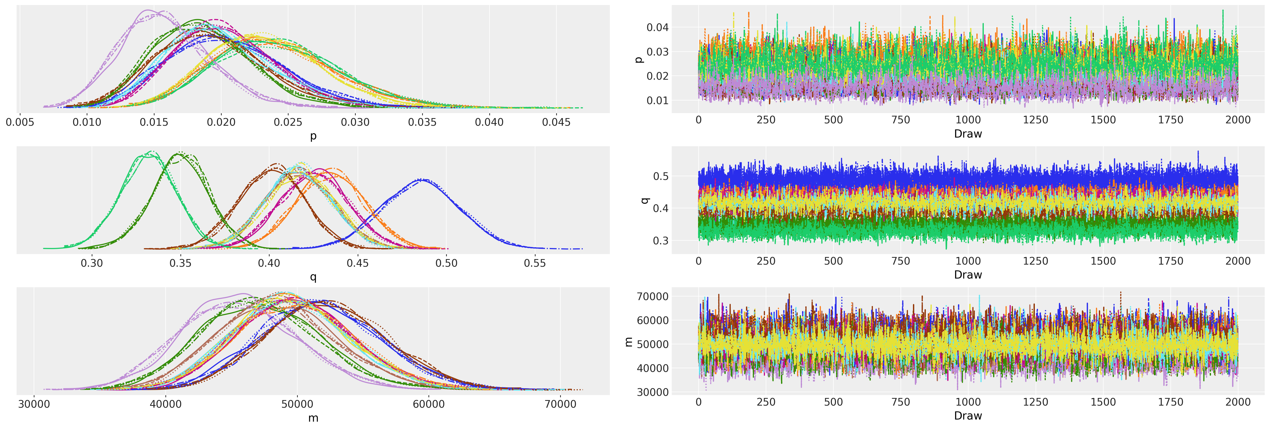
Overall, the diagnostics and trace look good.

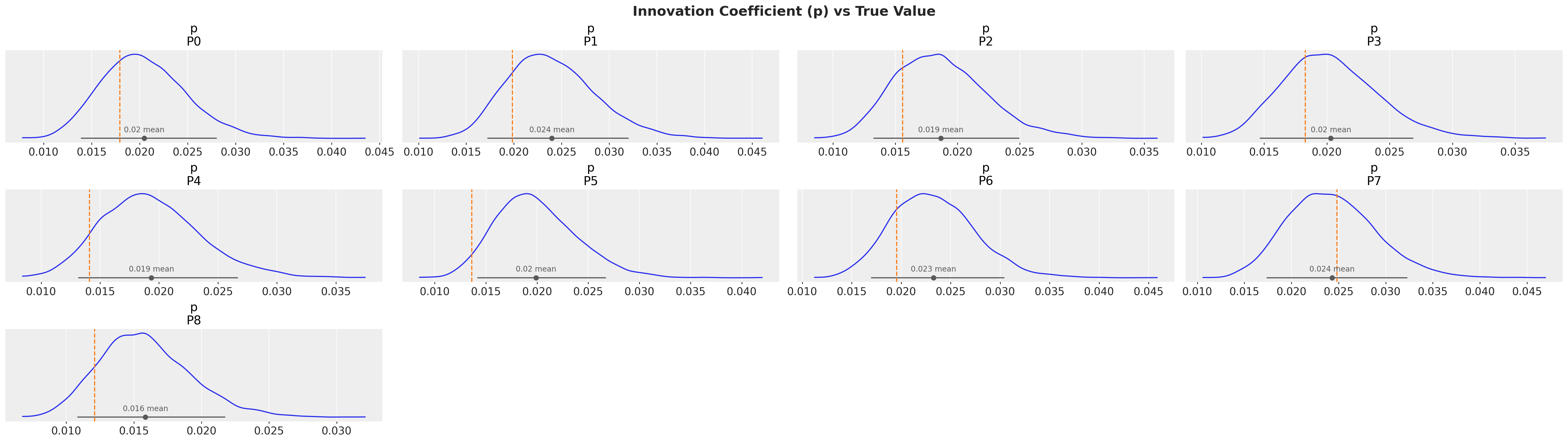
Next, we look into the posterior distributions of the parameters.

azp.plot_dist(xr.Dataset({"p": idata.posterior["p"]}))

fig = plt.gcf()
for ax, true_p in zip(fig.axes, prior_draw["p"].to_numpy(), strict=False):
    ax.axvline(true_p, color="C1", linestyle="--")

fig.suptitle(
    "Innovation Coefficient (p) vs True Value",
    fontsize=18,
    fontweight="bold",
);

azp.plot_dist(xr.Dataset({"q": idata.posterior["q"]}))

fig = plt.gcf()
for ax, true_q in zip(fig.axes, prior_draw["q"].to_numpy(), strict=False):
    ax.axvline(true_q, color="C1", linestyle="--")

fig.suptitle(
    "Imitation Coefficient (q) vs True Value",
    fontsize=18,
    fontweight="bold",
);

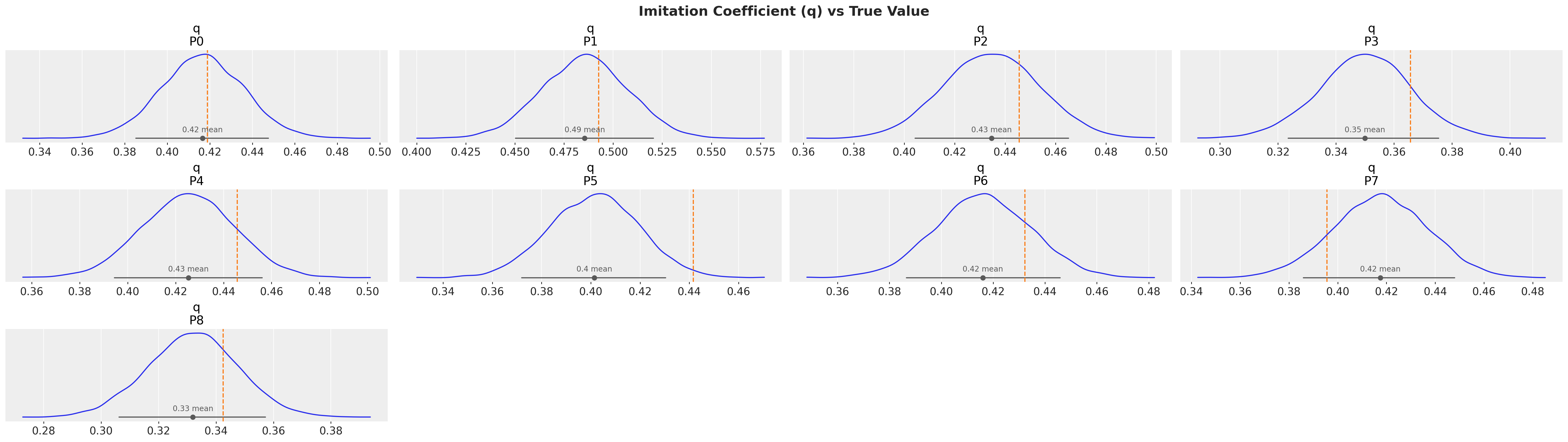
We do see some heterogeneity in the parameters, but the pooled posterior concentrates around the true per-product values (dashed lines) used to generate the data.

Examining Posterior Predictions for Specific Products

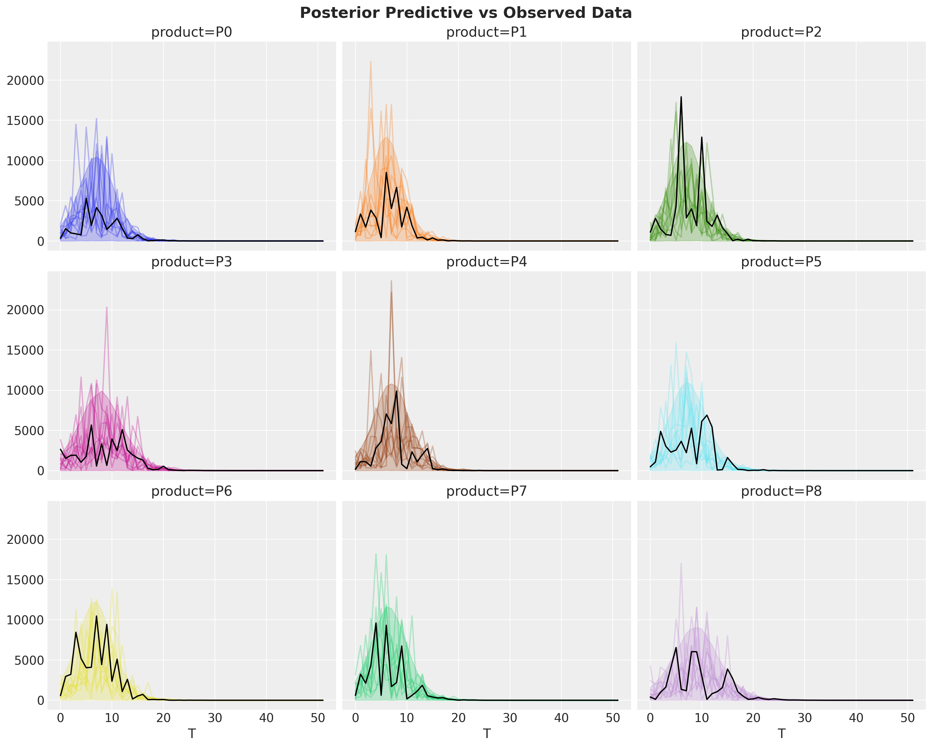
Let’s look at the posterior predictive distributions to see how well our model captures the simulated data.

fig, axes = plt.subplots(
    nrows=3, ncols=3, figsize=(15, 12), sharex=True, sharey=True, layout="constrained"
)

idata["posterior_predictive"]["y"].pipe(plot_curve, {"T"}, axes=axes)

for i, ax in enumerate(axes.flatten()):
    ax.plot(T, bass_data[:, i], color="black")

fig.suptitle("Posterior Predictive vs Observed Data", fontsize=18, fontweight="bold");

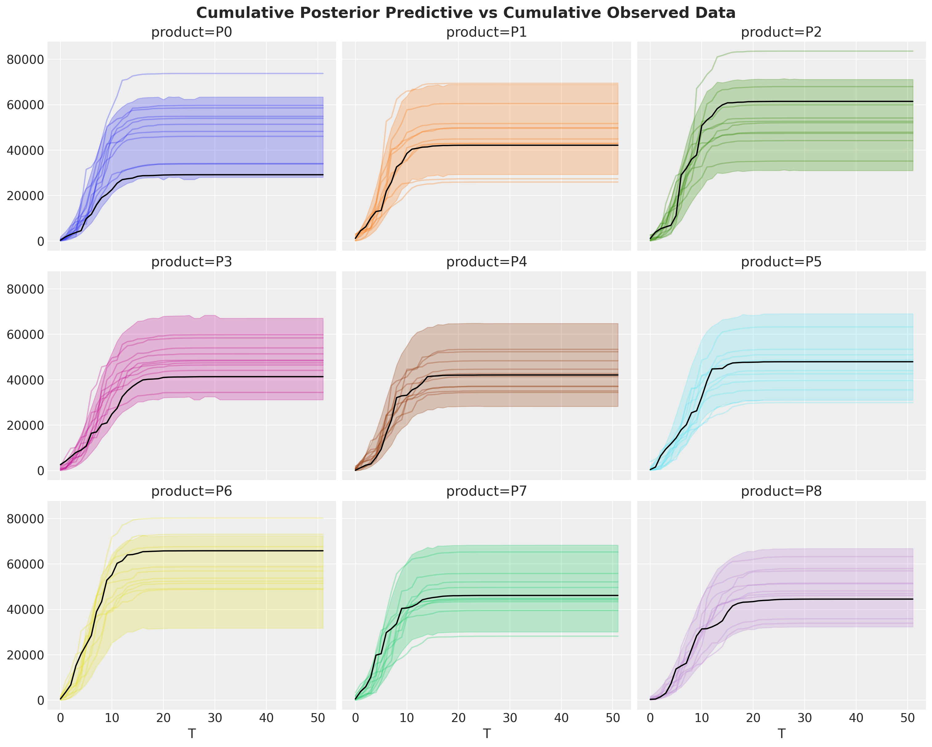
fig, axes = plt.subplots(
    nrows=3, ncols=3, figsize=(15, 12), sharex=True, sharey=True, layout="constrained"
)

idata["posterior_predictive"]["y"].cumsum(dim="T").pipe(plot_curve, {"T"}, axes=axes)

for i, ax in enumerate(axes.flatten()):
    ax.plot(T, bass_data[:, i].cumsum(), color="black")

fig.suptitle(
    "Cumulative Posterior Predictive vs Cumulative Observed Data",
    fontsize=18,
    fontweight="bold",
);

azp.plot_dist(xr.Dataset({"m": idata.posterior["m"]}))

fig = plt.gcf()
for ax, true_m in zip(fig.axes, prior_draw["m"].to_numpy(), strict=False):
    ax.axvline(true_m, color="C1", linestyle="--")

fig.suptitle(
    "Estimated Market Cap (m) vs True Value",
    fontsize=18,
    fontweight="bold",
);

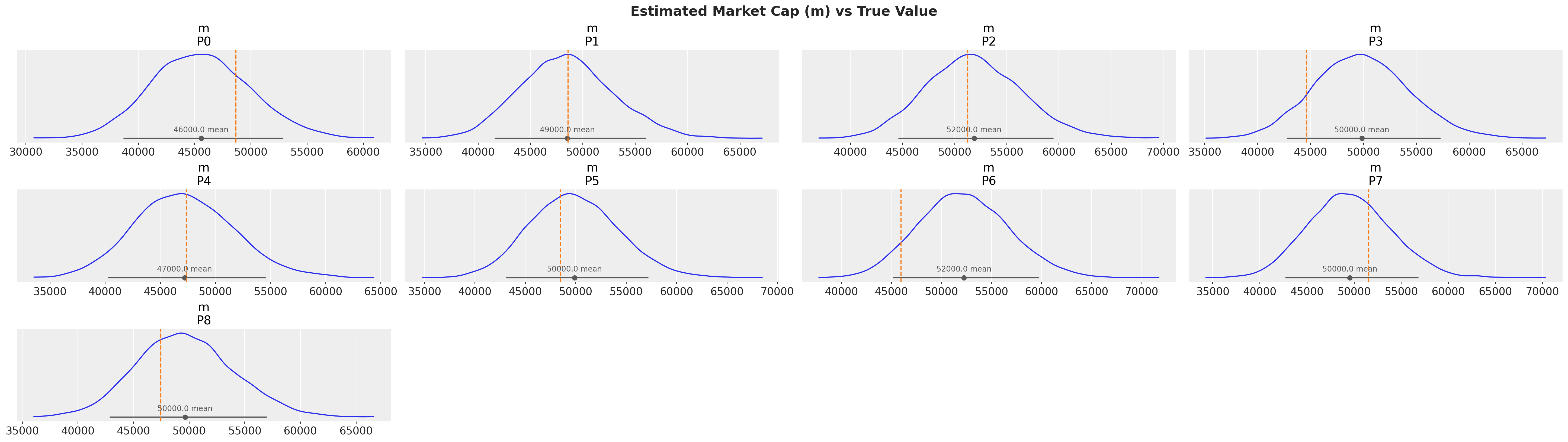
Overall, the model does a good job of capturing the data.

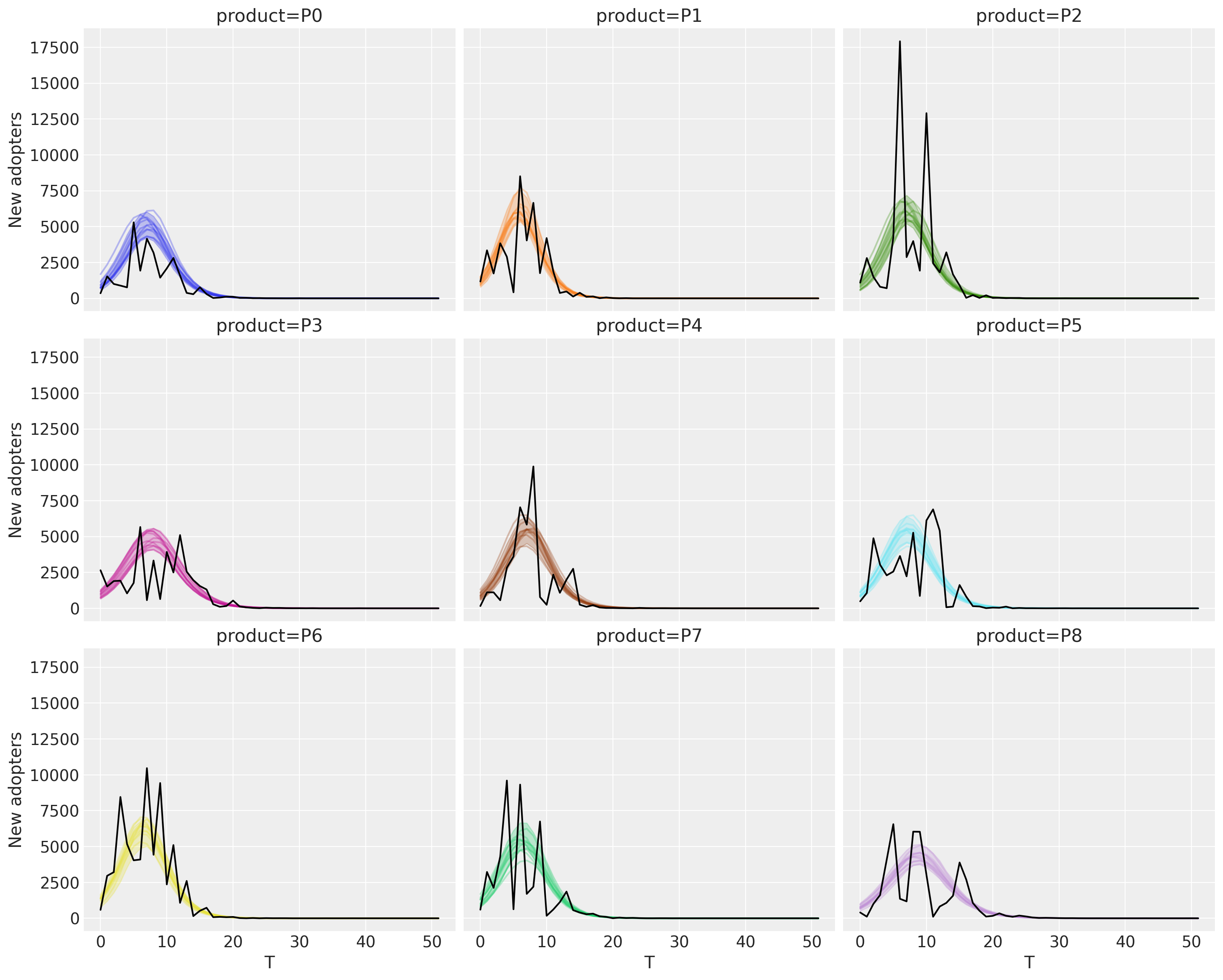
Next, we look into the adopters, which represent the expected value of the likelihood.

fig, axes = model.plot_adoption_curve(subplot_kwargs={"ncols": 3, "figsize": (15, 12)})

fig.suptitle("Adopters vs Observed Data", fontsize=18, fontweight="bold");

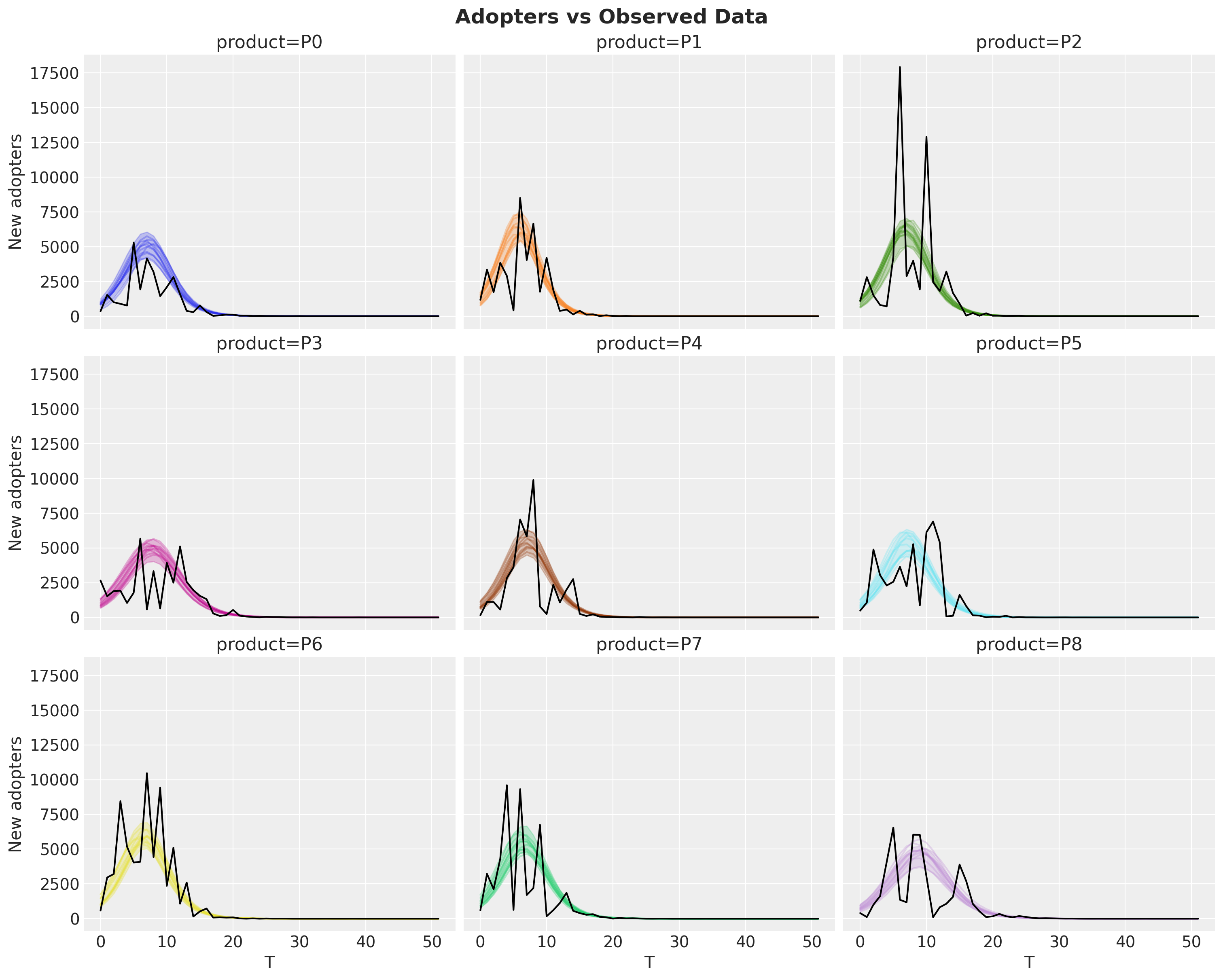
This show the fit is indeed quite reasonable.

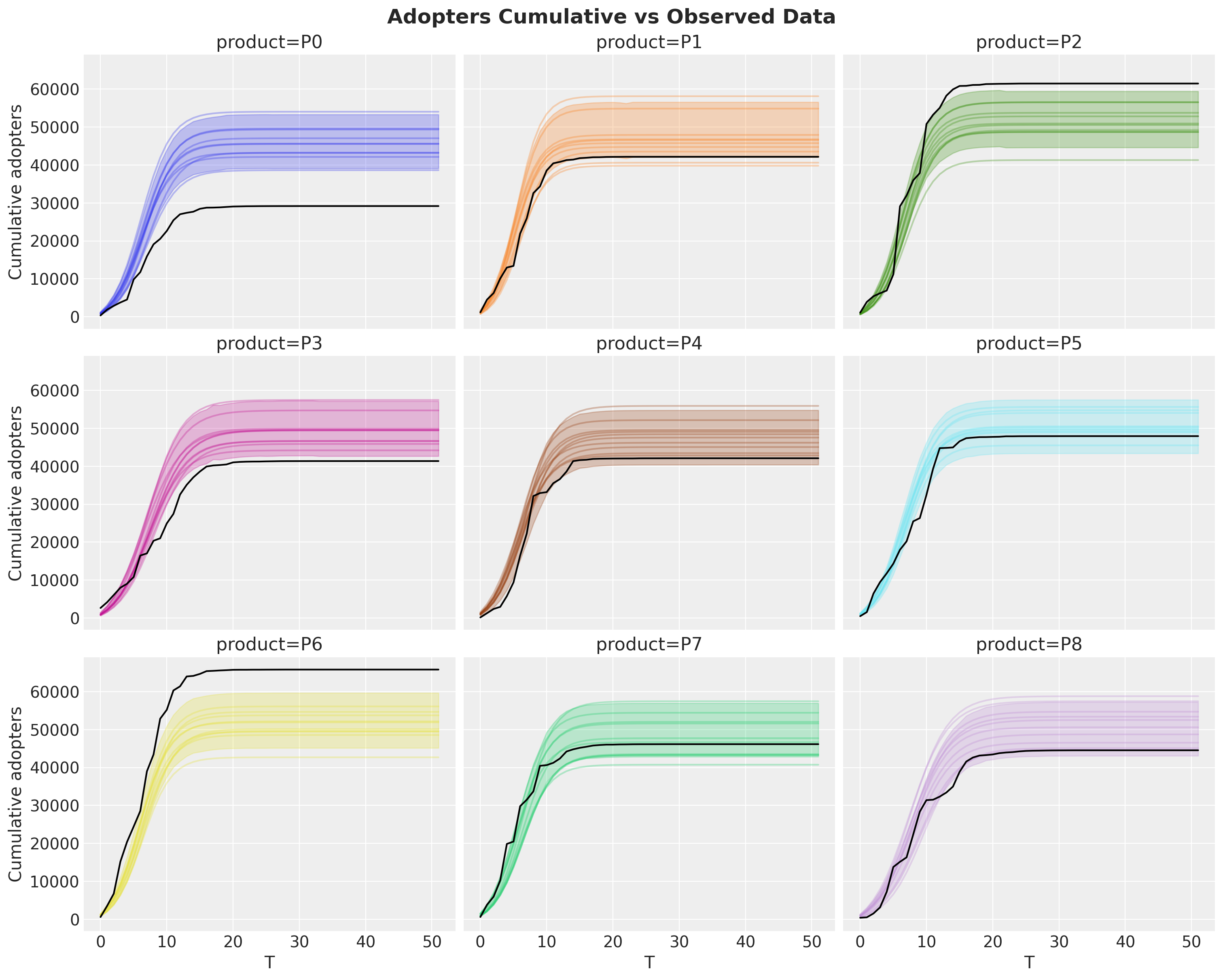
We can also evaluate the model goodness by looking into the cumulative data:

Note

Remember that the adopters is the mean of the distribution so we see some cumulative curves above and some below.

Look at the idata["posterior_predictive"]["y"] for the observed data.

fig, axes = model.plot_cumulative(subplot_kwargs={"ncols": 3, "figsize": (15, 12)})

fig.suptitle("Adopters Cumulative vs Observed Data", fontsize=18, fontweight="bold");

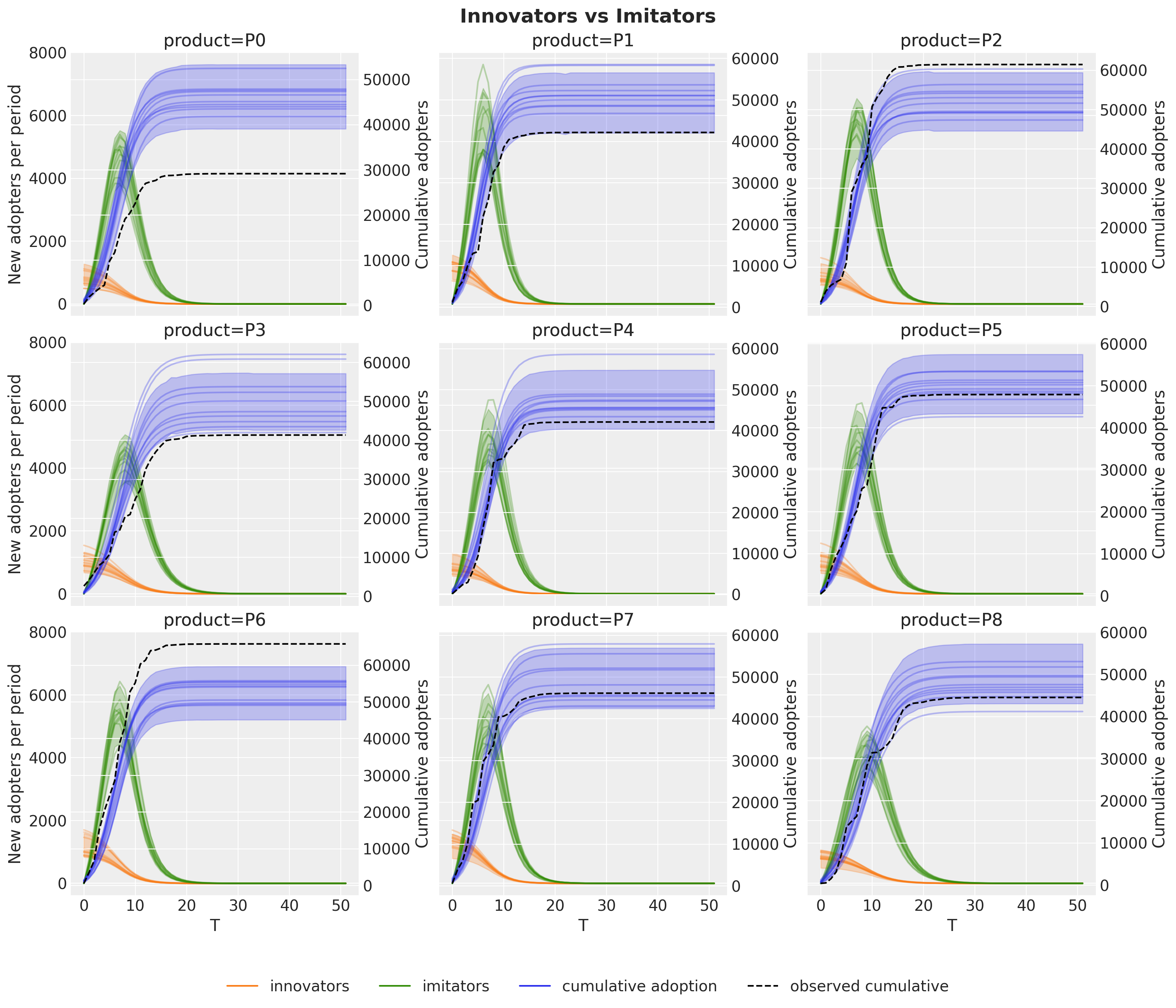
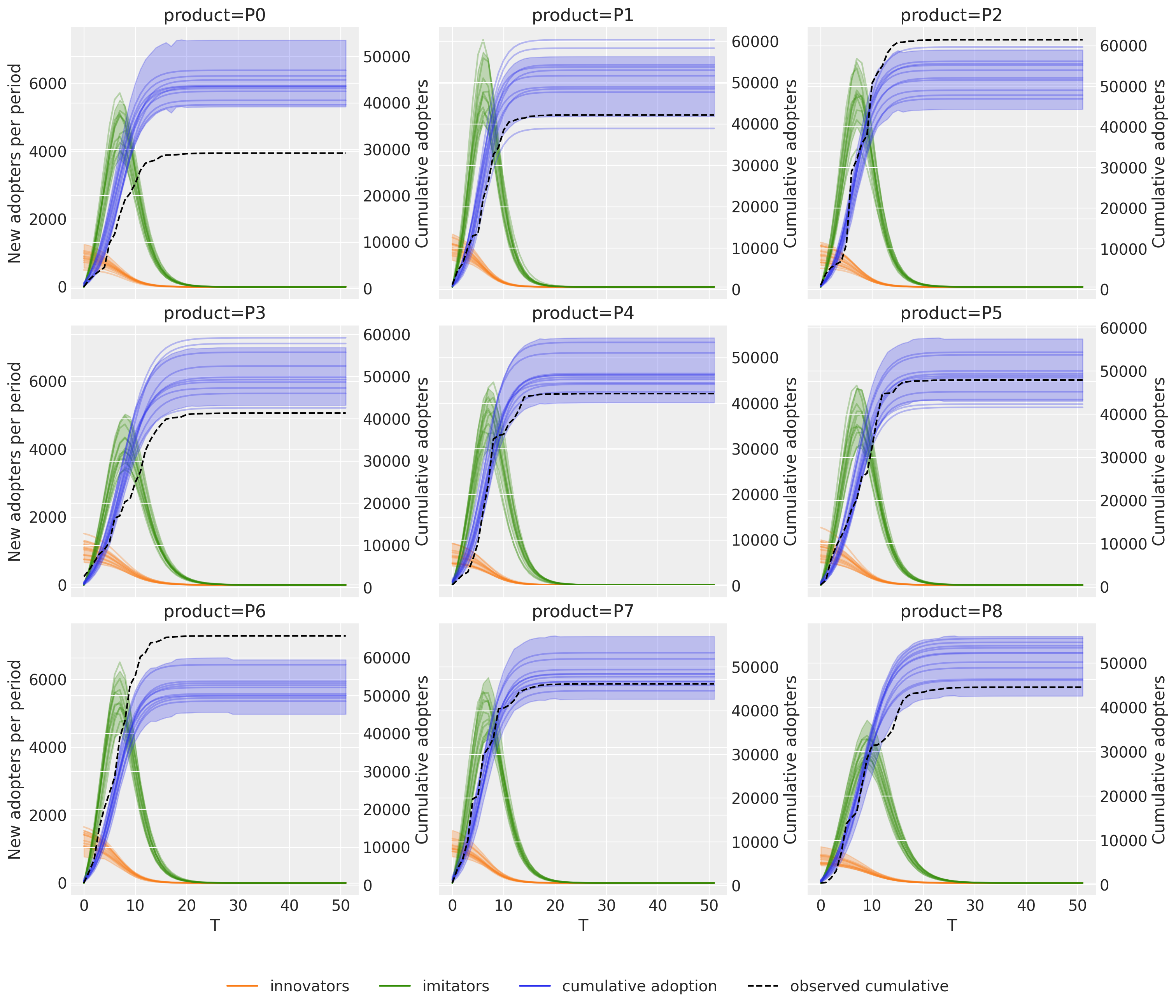
We can enhance this view by looking into the components of the model: innovators and imitators (in orange and green, respectively). The per-period components go on the left y-axis and the cumulative adoption on a twin right y-axis, since they live on very different scales.

fig, axes = model.plot_decomposition(subplot_kwargs={"ncols": 3, "figsize": (15, 12)})

fig.suptitle("Innovators vs Imitators", fontsize=18, fontweight="bold");

Finally, we can inspect the peak of the adoption curve. plot_peak forwards to arviz_plots.plot_dist(), so it takes col_wrap and figure_kwargs rather than the subplot_kwargs used by the other plotting methods.

fig, axes = model.plot_peak(col_wrap=3, figure_kwargs={"figsize": (15, 8)})

fig.suptitle("Peak", fontsize=18, fontweight="bold");

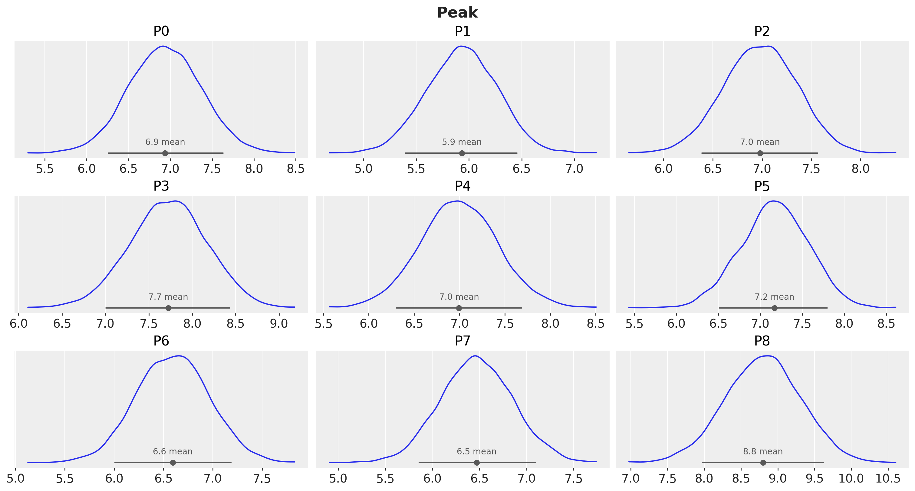
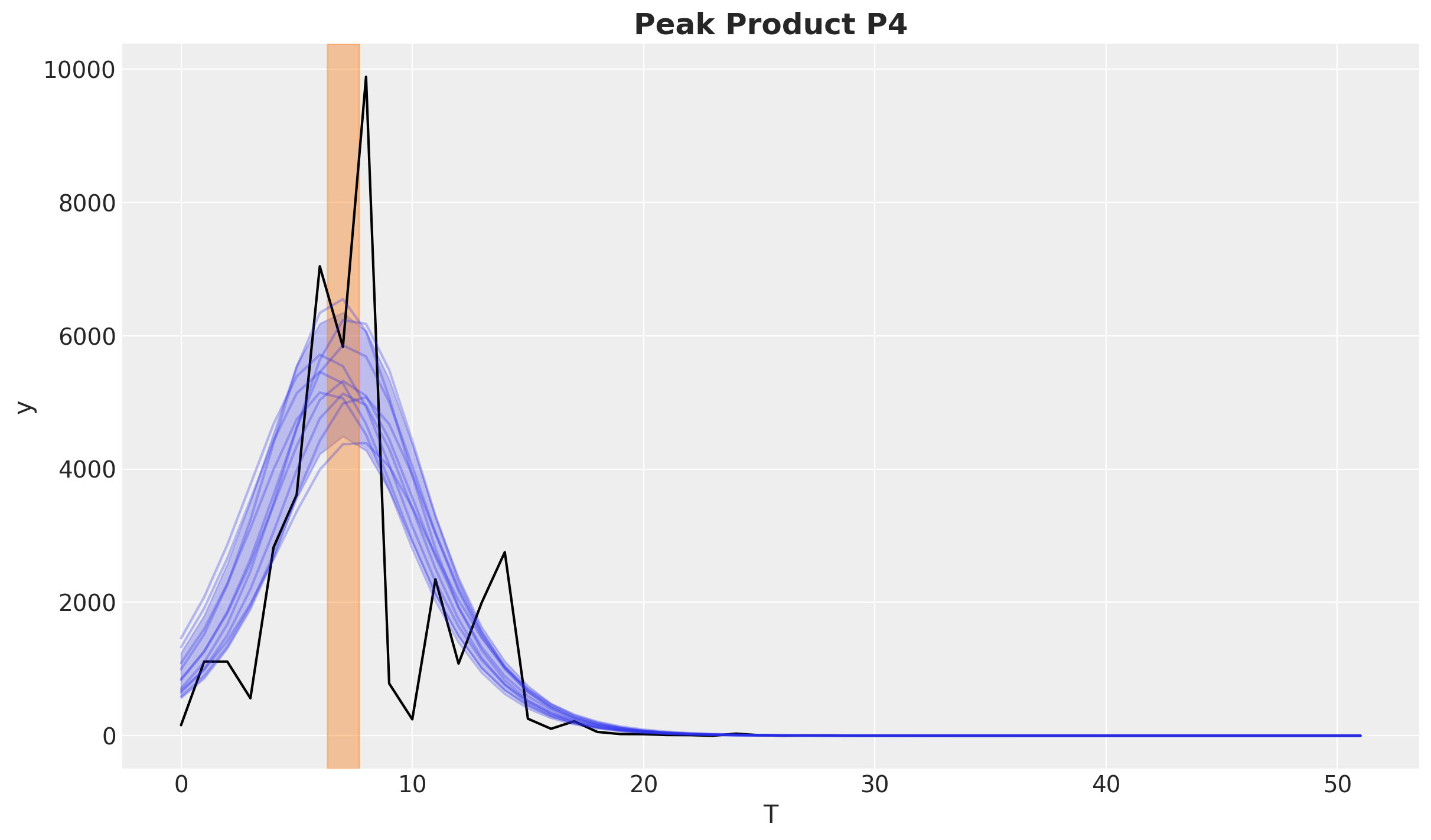
This fits the observed data quite well. Let’s see for example the product P4.

fig, ax = plt.subplots()

product_id = 4

bass_data[:, product_id].plot(ax=ax, color="black")

idata["posterior"]["adopters"].sel(product=f"P{product_id}").pipe(
    plot_curve, {"T"}, axes=ax
)

peak_hdi = az.hdi(idata["posterior"]["peak"].sel(product=f"P{product_id}"))
ax.axvspan(
    peak_hdi.sel(ci_bound="lower").item(),
    peak_hdi.sel(ci_bound="upper").item(),
    color="C1",
    alpha=0.4,
)

ax.set_title(f"Peak Product {products[product_id]}", fontsize=18, fontweight="bold");

Forecasting Beyond the Observed Window

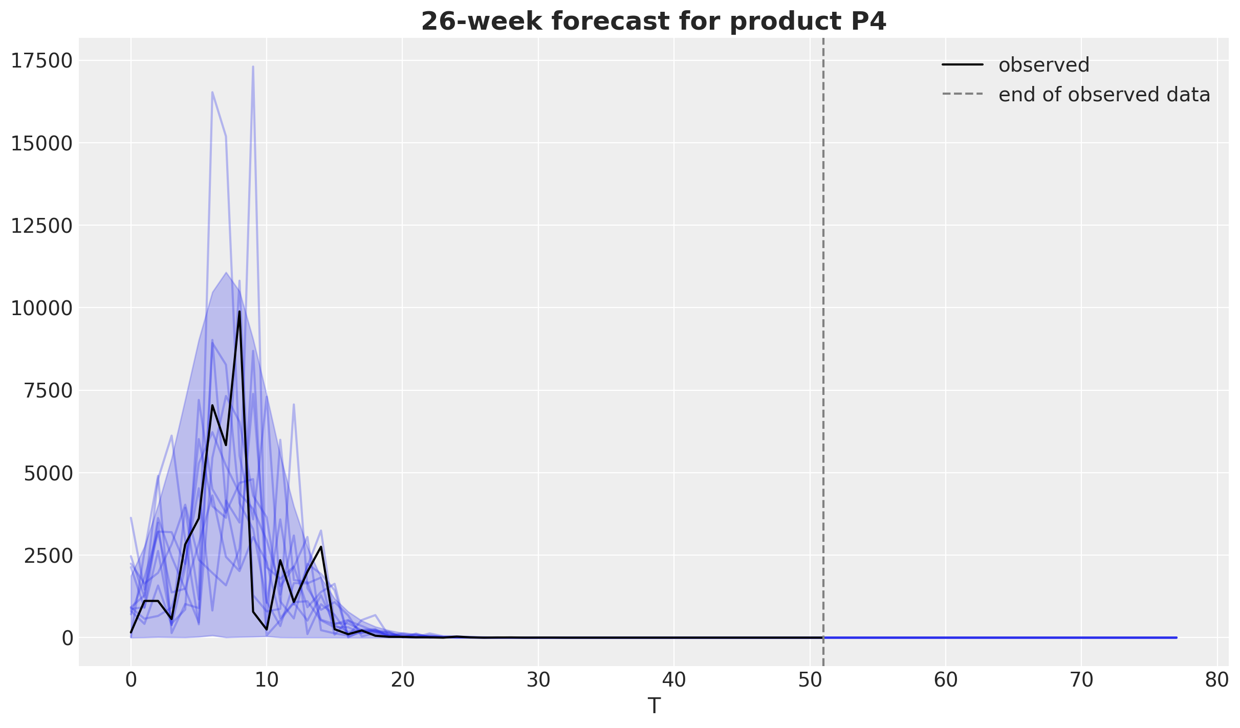
The sample_posterior_predictive method accepts new data with a different time range than the one used for fitting. Passing an extended T coordinate produces an out-of-sample forecast: the posterior of \(m\), \(p\) and \(q\) stays fixed and the adoption curve is evaluated over the new time points.

T_extended = np.arange(len(T) + 26)

forecast = model.sample_posterior_predictive(
    X=xr.Dataset(coords={"T": T_extended}),
    extend_idata=False,
    random_seed=rng,
)

fig, ax = plt.subplots()

forecast.sel(product="P4").pipe(plot_curve, {"T"}, axes=ax, legend=False)
(observed_line,) = ax.plot(
    T, bass_data.sel(product="P4"), color="black", label="observed"
)
cutoff_line = ax.axvline(
    int(T.max()), color="gray", linestyle="--", label="end of observed data"
)
ax.legend(handles=[observed_line, cutoff_line], loc="upper right")
ax.set_title("26-week forecast for product P4", fontsize=18, fontweight="bold");

Sampling: [y]

Save and Load the Model

The fitted model can be stored as a single NetCDF file and restored later. The file contains the posterior together with the model configuration (the priors) and the data used for fitting, so the loaded model is ready for posterior analysis, plotting, and posterior predictive sampling.

model_path = f"{tempfile.mkdtemp()}/bass_model.nc"
model.save(model_path)

loaded_model = BassModel.load(model_path)

display(az.summary(loaded_model.idata, var_names=["p", "q"]).head())

# The config round-trips as Prior/Scaled objects, not plain dicts:
loaded_model.model_config["m"]

	mean	sd	eti89_lb	eti89_ub	ess_bulk	ess_tail	r_hat	mcse_mean	mcse_sd
p[P0]	0.0205	0.00441	0.014	0.028	6490	5644	1.00	5.5e-05	4.2e-05
p[P1]	0.024	0.00462	0.017	0.032	8216	5942	1.00	5.1e-05	3.8e-05
p[P2]	0.01866	0.0037	0.013	0.025	7329	6184	1.00	4.3e-05	3.2e-05
p[P3]	0.02032	0.00383	0.015	0.027	7339	5946	1.00	4.5e-05	3.5e-05
p[P4]	0.0194	0.00423	0.013	0.027	7077	5721	1.00	5e-05	3.9e-05

<pymc_extras.prior.Scaled at 0x7ff49e2596d0>

MLflow Integration

The MLflow autologging from pymc_marketing.mlflow supports the Bass model through the log_bass flag. Enabling it patches BassModel.fit so every fit inside an MLflow run logs the model configuration (the priors for m, p, q and the likelihood), the sampler diagnostics, the model graph, and the resulting InferenceData as artifacts. Figures from the plotting methods can be logged with mlflow.log_figure.

We refit the model with a lighter sampler configuration to keep the demo fast.

import mlflow

import pymc_marketing.mlflow

pymc_marketing.mlflow.autolog(log_bass=True)

mlflow_dir = tempfile.mkdtemp()
mlflow.set_tracking_uri(f"sqlite:///{mlflow_dir}/mlflow.db")
mlflow.set_experiment(
    experiment_id=mlflow.create_experiment(
        "bass-model", artifact_location=f"{mlflow_dir}/artifacts"
    )
)

mlflow_model = BassModel(
    model_config=priors,
    sampler_config={
        "tune": 1_000,
        "draws": 1_000,
        "chains": 2,
        "nuts_sampler": "nutpie",
        "compile_kwargs": {"mode": "NUMBA"},
    },
)

with mlflow.start_run():
    mlflow_model.fit(data=observed_ds, random_seed=rng)

    fig, _ = mlflow_model.plot_adoption_curve(
        subplot_kwargs={"ncols": 3, "figsize": (15, 12)}
    )
    mlflow.log_figure(fig, "adoption_curve.png")

    fig, _ = mlflow_model.plot_decomposition(
        subplot_kwargs={"ncols": 3, "figsize": (15, 12)}
    )
    mlflow.log_figure(fig, "decomposition.png")

2026/07/30 21:55:36 INFO mlflow.store.db.utils: Creating initial MLflow database tables...

2026/07/30 21:55:36 INFO mlflow.store.db.utils: Updating database tables

NUTS[nutpie]: [m_unscaled, p, q]

%load_ext watermark
%watermark -n -u -v -iv -w -p nutpie,pymc_marketing,pytensor

Last updated: Thu, 30 Jul 2026

Python implementation: CPython
Python version       : 3.13.12
IPython version      : 9.15.0

nutpie        : 0.16.10
pymc_marketing: 1.0.0.dev0
pytensor      : 3.0.7

arviz         : 1.2.0
arviz_plots   : 1.2.0
matplotlib    : 3.10.9
mlflow        : 3.14.0
numpy         : 2.4.6
pandas        : 2.3.3
pymc          : 6.0.1
pymc_extras   : 0.12.2.dev1+gee8cc37df
pymc_marketing: 1.0.0.dev0
xarray        : 2026.4.0

Watermark: 2.6.0